Data visualization is an essential tool for understanding, analyzing, and communicating the behavior of energy-based models. This guide covers various visualization techniques available in TorchEBM to help you gain insights into energy landscapes, sampling processes, and model performance.
Visualizing energy landscapes is crucial for understanding the structure of the probability distribution you're working with. TorchEBM provides utilities to create both 2D and 3D visualizations of energy functions.
importtorchimportnumpyasnpimportmatplotlib.pyplotaspltfromtorchebm.coreimportDoubleWellEnergy# Create the energy functionenergy_fn=DoubleWellEnergy(barrier_height=2.0)# Create a grid for visualizationx=np.linspace(-3,3,100)y=np.linspace(-3,3,100)X,Y=np.meshgrid(x,y)Z=np.zeros_like(X)# Compute energy valuesforiinrange(X.shape[0]):forjinrange(X.shape[1]):point=torch.tensor([X[i,j],Y[i,j]],dtype=torch.float32).unsqueeze(0)Z[i,j]=energy_fn(point).item()# Create 3D surface plotfig=plt.figure(figsize=(10,8))ax=fig.add_subplot(111,projection='3d')surf=ax.plot_surface(X,Y,Z,cmap='viridis',alpha=0.8)ax.set_xlabel('x')ax.set_ylabel('y')ax.set_zlabel('Energy')ax.set_title('Double Well Energy Landscape')plt.colorbar(surf,ax=ax,shrink=0.5,aspect=5)plt.tight_layout()plt.show()
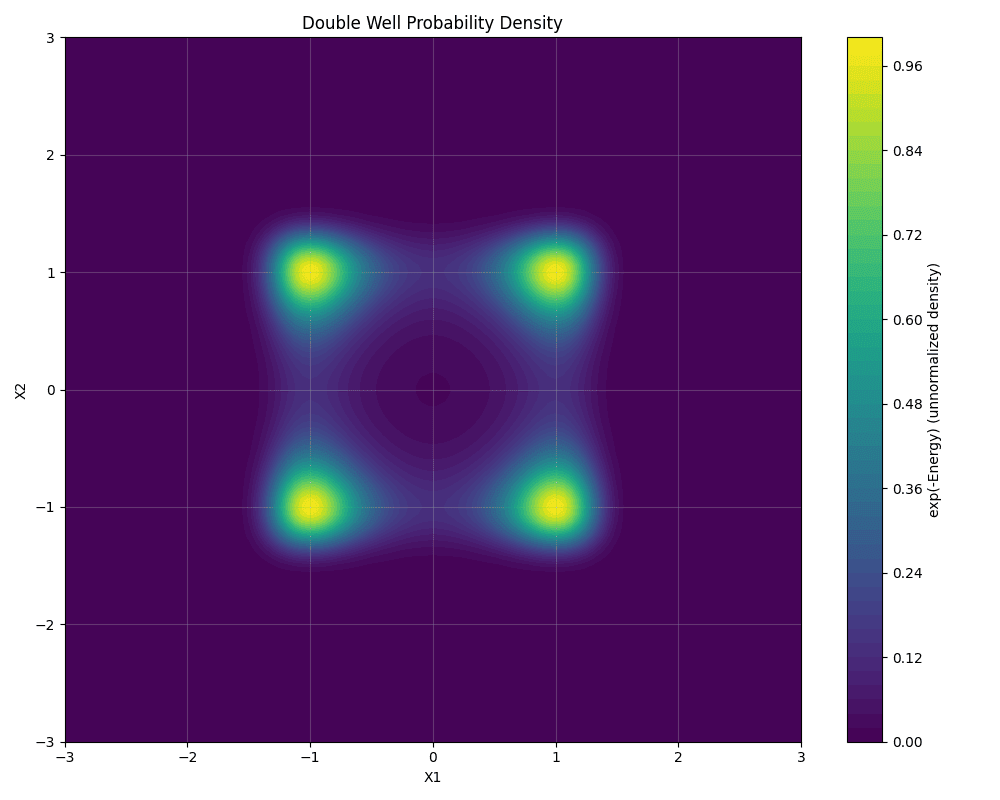
importtorchimportnumpyasnpimportmatplotlib.pyplotaspltfromtorchebm.coreimportDoubleWellEnergy# Create the energy functionenergy_fn=DoubleWellEnergy(barrier_height=2.0)# Create a grid for visualizationgrid_size=100plot_range=3.0x_coords=np.linspace(-plot_range,plot_range,grid_size)y_coords=np.linspace(-plot_range,plot_range,grid_size)X,Y=np.meshgrid(x_coords,y_coords)Z=np.zeros_like(X)# Compute energy valuesforiinrange(X.shape[0]):forjinrange(X.shape[1]):point=torch.tensor([X[i,j],Y[i,j]],dtype=torch.float32).unsqueeze(0)Z[i,j]=energy_fn(point).item()# Convert energy to probability density (unnormalized)# Subtract max for numerical stability before exponentiatinglog_prob_values=-Zlog_prob_values=log_prob_values-np.max(log_prob_values)prob_density=np.exp(log_prob_values)# Create contour plotplt.figure(figsize=(10,8))contour=plt.contourf(X,Y,prob_density,levels=50,cmap='viridis')plt.colorbar(label='exp(-Energy) (unnormalized density)')plt.xlabel('X1')plt.ylabel('X2')plt.title('Double Well Probability Density')plt.grid(True,alpha=0.3)plt.tight_layout()plt.show()
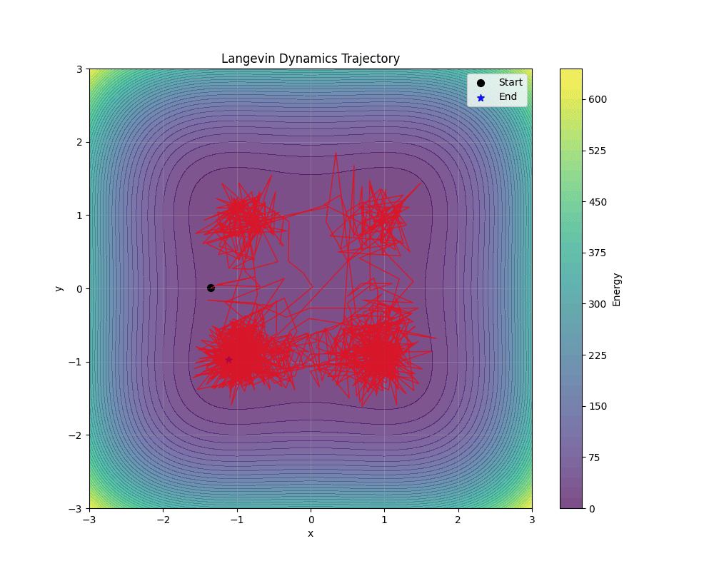
fromtorchebm.coreimportDoubleWellEnergy,LinearScheduler,WarmupSchedulerfromtorchebm.samplersimportLangevinDynamics# Create energy function and samplerenergy_fn=DoubleWellEnergy(barrier_height=5.0)# Define a cosine scheduler for the Langevin dynamicsscheduler_linear=LinearScheduler(initial_value=0.05,final_value=0.03,total_steps=100)scheduler=WarmupScheduler(main_scheduler=scheduler_linear,warmup_steps=10,warmup_init_factor=0.01)sampler=LangevinDynamics(energy_function=energy_fn,step_size=scheduler)# Initial pointinitial_point=torch.tensor([[-2.0,0.0]],dtype=torch.float32)# Run sampling and get trajectorytrajectory=sampler.sample(x=initial_point,dim=2,n_steps=1000,return_trajectory=True)# Background energy landscapex=np.linspace(-3,3,100)y=np.linspace(-3,3,100)X,Y=np.meshgrid(x,y)Z=np.zeros_like(X)foriinrange(X.shape[0]):forjinrange(X.shape[1]):point=torch.tensor([X[i,j],Y[i,j]],dtype=torch.float32).unsqueeze(0)Z[i,j]=energy_fn(point).item()# Visualizeplt.figure(figsize=(10,8))plt.contourf(X,Y,Z,50,cmap='viridis',alpha=0.7)plt.colorbar(label='Energy')# Extract trajectory coordinatestraj_x=trajectory[0,:,0].numpy()traj_y=trajectory[0,:,1].numpy()# Plot trajectoryplt.plot(traj_x,traj_y,'r-',linewidth=1,alpha=0.7)plt.scatter(traj_x[0],traj_y[0],c='black',s=50,marker='o',label='Start')plt.scatter(traj_x[-1],traj_y[-1],c='blue',s=50,marker='*',label='End')plt.xlabel('x')plt.ylabel('y')plt.title('Langevin Dynamics Trajectory')plt.legend()plt.grid(True,alpha=0.3)plt.savefig('langevin_trajectory.png')plt.show()
importtorchimportnumpyasnpimportmatplotlib.pyplotaspltfromtorchebm.coreimportRastriginEnergyfromtorchebm.samplersimportLangevinDynamics# Set random seed for reproducibilitytorch.manual_seed(44)np.random.seed(43)# Create energy function and samplerenergy_fn=RastriginEnergy(a=10.0)sampler=LangevinDynamics(energy_function=energy_fn,step_size=0.008)# Parameters for samplingdim=2n_steps=1000num_chains=5# Generate random starting pointsinitial_points=torch.randn(num_chains,dim)*3# Run sampling and get trajectorytrajectories=sampler.sample(x=initial_points,dim=dim,n_samples=num_chains,n_steps=n_steps,return_trajectory=True)# Create background contourx=np.linspace(-5,5,100)y=np.linspace(-5,5,100)X,Y=np.meshgrid(x,y)Z=np.zeros_like(X)print(trajectories.shape)foriinrange(X.shape[0]):forjinrange(X.shape[1]):point=torch.tensor([X[i,j],Y[i,j]],dtype=torch.float32).unsqueeze(0)Z[i,j]=energy_fn(point).item()# Plot contourplt.figure(figsize=(12,10))contour=plt.contourf(X,Y,Z,50,cmap='viridis',alpha=0.7)plt.colorbar(label='Energy')# Plot each trajectory with a different colorcolors=['red','blue','green','orange','purple']foriinrange(num_chains):traj_x=trajectories[i,:,0].numpy()traj_y=trajectories[i,:,1].numpy()plt.plot(traj_x,traj_y,alpha=0.7,linewidth=1,c=colors[i],label=f'Chain {i+1}')# Mark start and end pointsplt.scatter(traj_x[0],traj_y[0],c='black',s=50,marker='o')plt.scatter(traj_x[-1],traj_y[-1],c=colors[i],s=100,marker='*')plt.xlabel('x')plt.ylabel('y')plt.title('Multiple Langevin Dynamics Sampling Chains on Rastrigin Potential')plt.legend()plt.tight_layout()plt.savefig('multiple_chains.png')plt.show()
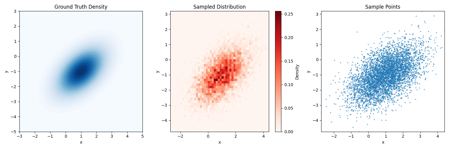
importtorchimportnumpyasnpimportmatplotlib.pyplotaspltfromscipyimportstatsfromtorchebm.coreimportGaussianEnergyfromtorchebm.samplersimportLangevinDynamics# Create a Gaussian energy functionmean=torch.tensor([1.0,-1.0])cov=torch.tensor([[1.0,0.5],[0.5,1.0]])energy_fn=GaussianEnergy(mean=mean,cov=cov)# Sample using Langevin dynamicssampler=LangevinDynamics(energy_function=energy_fn,step_size=0.01)# Generate samplesn_samples=5000burn_in=200# Initialize random samplesx=torch.randn(n_samples,2)# Perform samplingsamples=sampler.sample(x=x,n_steps=1000,burn_in=burn_in,return_trajectory=False)# Convert to numpy for visualizationsamples_np=samples.numpy()mean_np=mean.numpy()cov_np=cov.numpy()# Create a grid for the ground truth densityx=np.linspace(-3,5,100)y=np.linspace(-5,3,100)X,Y=np.meshgrid(x,y)pos=np.dstack((X,Y))# Calculate multivariate normal PDFrv=stats.multivariate_normal(mean_np,cov_np)Z=rv.pdf(pos)# Create figure with multiple plotsfig=plt.figure(figsize=(15,5))# Ground truth contourax1=fig.add_subplot(131)ax1.contourf(X,Y,Z,50,cmap='Blues')ax1.set_title('Ground Truth Density')ax1.set_xlabel('x')ax1.set_ylabel('y')# Sample density (using kernel density estimation)ax2=fig.add_subplot(132)h=ax2.hist2d(samples_np[:,0],samples_np[:,1],bins=50,cmap='Reds',density=True)plt.colorbar(h[3],ax=ax2,label='Density')ax2.set_title('Sampled Distribution')ax2.set_xlabel('x')ax2.set_ylabel('y')# Scatter plot of samplesax3=fig.add_subplot(133)ax3.scatter(samples_np[:,0],samples_np[:,1],alpha=0.5,s=3)ax3.set_title('Sample Points')ax3.set_xlabel('x')ax3.set_ylabel('y')ax3.set_xlim(ax2.get_xlim())ax3.set_ylim(ax2.get_ylim())plt.tight_layout()plt.savefig('distribution_comparison_updated.png')plt.show()
importnumpyasnpimporttorchimportmatplotlib.pyplotaspltfromtorchebm.coreimportDoubleWellEnergy,GaussianEnergy,CosineSchedulerfromtorchebm.samplersimportLangevinDynamicsSAMPLER_STEP_SIZE=CosineScheduler(initial_value=1e-2,final_value=1e-3,total_steps=50)SAMPLER_NOISE_SCALE=CosineScheduler(initial_value=2e-1,final_value=1e-2,total_steps=50)# Create energy function and samplerenergy_fn=GaussianEnergy(mean=torch.tensor([0.0,0.0]),cov=torch.eye(2)*0.5)sampler=LangevinDynamics(energy_function=energy_fn,step_size=SAMPLER_STEP_SIZE,noise_scale=SAMPLER_NOISE_SCALE)# Parameters for samplingdim=2n_steps=200initial_point=torch.tensor([[-2.0,0.0]],dtype=torch.float32)# Track the energy during samplingenergy_values=[]current_sample=initial_point.clone()# Run the sampling steps and store each energyforiinrange(n_steps):noise=torch.randn_like(current_sample)current_sample=sampler.langevin_step(current_sample,noise)energy_values.append(energy_fn(current_sample).item())# Convert to numpy for plottingenergy_values_np=np.array(energy_values)# Plot energy evolutionplt.figure(figsize=(10,6))plt.plot(energy_values_np)plt.xlabel('Step')plt.ylabel('Energy')plt.title('Energy Evolution During Langevin Dynamics Sampling')plt.grid(True,alpha=0.3)plt.tight_layout()plt.savefig('energy_evolution_updated.png')plt.show()
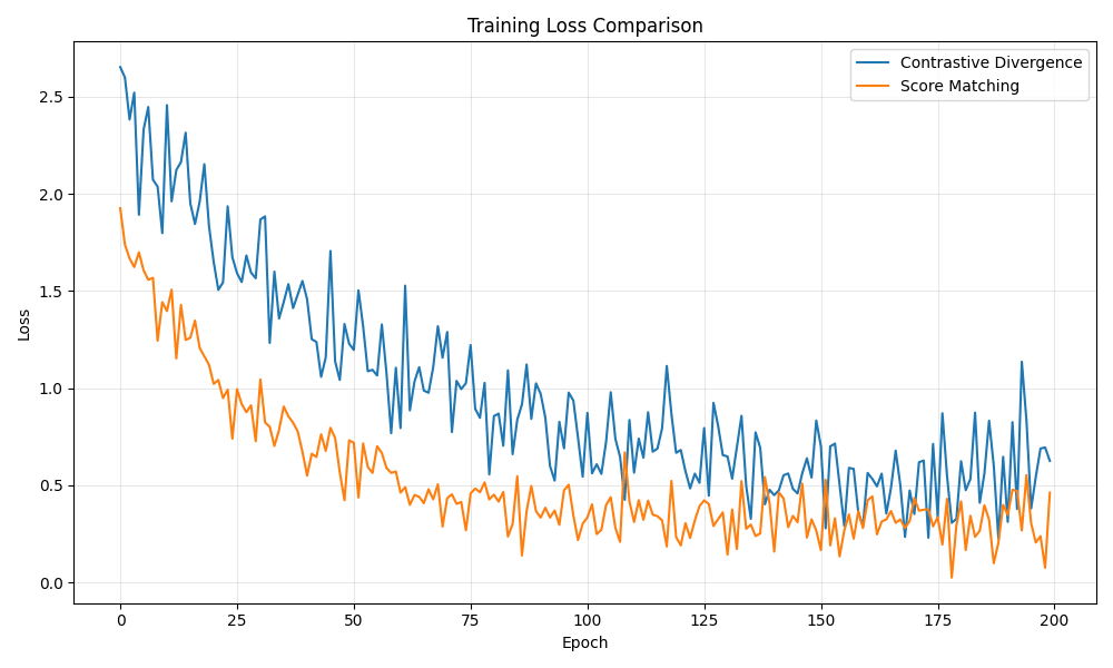
Visualizing Training Progress with Different Loss Functions
You can also visualize how different loss functions affect the training dynamics:
importtorchimportnumpyasnpimportmatplotlib.pyplotaspltfromtorchebm.coreimportBaseEnergyFunctionfromtorchebm.lossesimportContrastiveDivergence,ScoreMatchingfromtorchebm.samplersimportLangevinDynamicsfromtorchebm.datasetsimportTwoMoonsDatasetimporttorch.nnasnnimporttorch.optimasoptim# Define a simple MLP energy functionclassMLPEnergy(BaseEnergyFunction):def__init__(self,input_dim,hidden_dim=64):super().__init__()self.network=nn.Sequential(nn.Linear(input_dim,hidden_dim),nn.SELU(),nn.Linear(hidden_dim,hidden_dim),nn.SELU(),nn.Linear(hidden_dim,1))defforward(self,x):returnself.network(x).squeeze(-1)# Training functiondeftrain_and_record_loss(loss_type,n_epochs=100):# Reset modelenergy_model=MLPEnergy(input_dim=2,hidden_dim=32).to(device)# Setup sampler and losssampler=LangevinDynamics(energy_function=energy_model,step_size=0.1,device=device)ifloss_type=='CD':loss_fn=ContrastiveDivergence(energy_function=energy_model,sampler=sampler,k_steps=10,persistent=True)elifloss_type=='SM':loss_fn=ScoreMatching(energy_function=energy_model,hutchinson_samples=5)optimizer=optim.Adam(energy_model.parameters(),lr=0.001)# Record losslosses=[]# Trainforepochinrange(n_epochs):epoch_loss=0.0forbatchindataloader:optimizer.zero_grad()loss=loss_fn(batch)loss.backward()optimizer.step()epoch_loss+=loss.item()avg_loss=epoch_loss/len(dataloader)losses.append(avg_loss)if(epoch+1)%10==0:print(f"{loss_type} - Epoch {epoch+1}/{n_epochs}, Loss: {avg_loss:.4f}")returnlosses# Setup data and devicedevice=torch.device("cuda"iftorch.cuda.is_available()else"cpu")dataset=TwoMoonsDataset(n_samples=1000,noise=0.1,device=device)dataloader=torch.utils.data.DataLoader(dataset,batch_size=64,shuffle=True)# Train with different loss functionscd_losses=train_and_record_loss('CD')sm_losses=train_and_record_loss('SM')# Plot lossesplt.figure(figsize=(10,6))plt.plot(cd_losses,label='Contrastive Divergence')plt.plot(sm_losses,label='Score Matching')plt.xlabel('Epoch')plt.ylabel('Loss')plt.title('Training Loss Comparison')plt.legend()plt.grid(True,alpha=0.3)plt.tight_layout()plt.savefig('loss_comparison.png')plt.show()
Effective visualization is key to understanding and debugging energy-based models. TorchEBM provides tools for visualizing energy landscapes, sampling trajectories, and model performance. These visualizations can help you gain insights into your models and improve their design and performance.
Remember to adapt these examples to your specific needs - you might want to visualize higher-dimensional spaces using dimensionality reduction techniques, or create specialized plots for your particular application.