Video World Models
The World Simulator Problem
Video generation has reached a peculiar inflection point. State-of-the-art diffusion models can synthesize remarkably realistic short clips, but they fundamentally cannot serve as world simulators. Why? Because they generate all frames simultaneously using bidirectional attention. The future affects the past.
This bidirectional design creates a hard constraint. If you want to generate frame 50, you must also generate frame 100 at the same time. There is no mechanism to produce frames on the fly as new conditions arrive. You cannot build an interactive game engine, a robotic planning module, or a live streaming system on top of a model that requires clairvoyance.
The goal of this post is to trace the path from slow, bidirectional video diffusion to fast, autoregressive world models. Along the way, I will cover the core ideas that make this transition possible.
We begin with the causality problem and how masking attention can convert a bidirectional model to a causal one . We then examine the train-test distribution mismatch that plagues autoregressive generation through the lens of three training paradigms: Teacher Forcing, Diffusion Forcing , and Self Forcing . We will see how MotionStream extends these ideas to motion-controlled, infinite-length streaming through attention sinks. We will take a closer look at distribution matching distillation , which compresses 50-step diffusion into 4 steps while preserving quality. We will look at Mixture of Contexts , a learnable sparse attention mechanism that gives the model minute-long memory without the quadratic cost. And we will touch on the emerging class of 4D world models that jointly predict geometry, appearance, and dynamics.
Throughout, I will try to connect these developments. The recurring theme is that video generation is fundamentally about compressing the past into a representation that predicts the future, and different architectural choices make different tradeoffs in this compression.
Causality in Video Diffusion
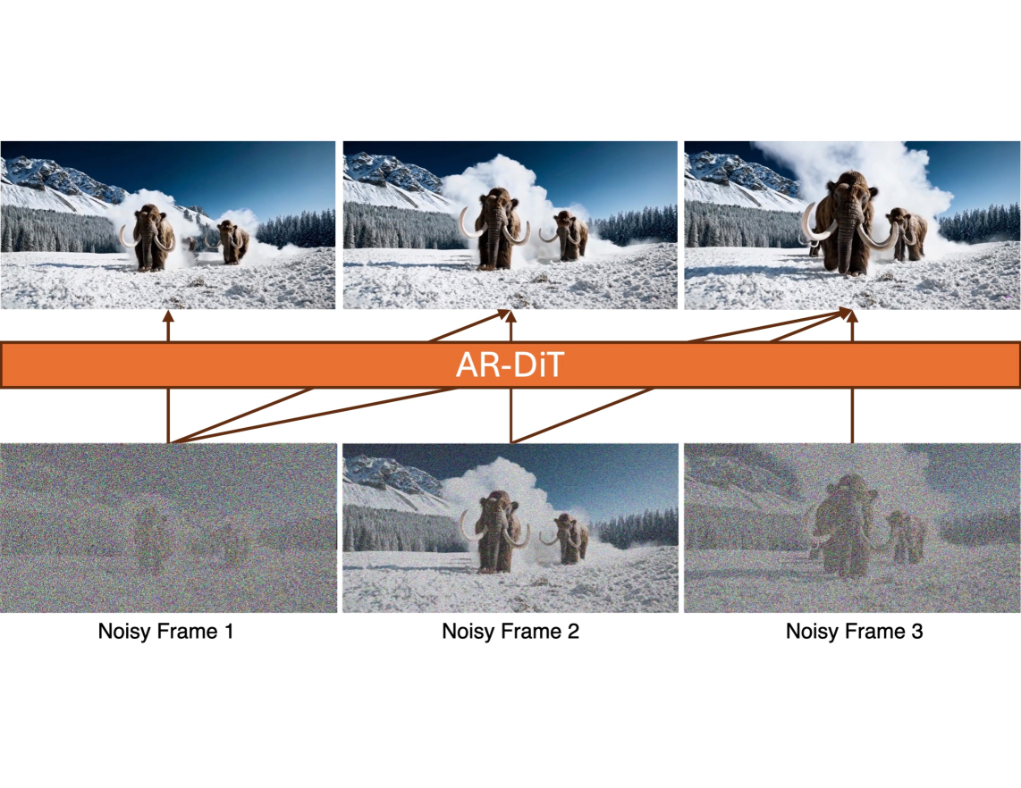
Standard video diffusion transformers process all frames together with bidirectional self-attention. Every token attends to every other token across space and time. This global receptive field is powerful for capturing coherence but has a fatal flaw for interactive applications. Generating a single frame requires the model to process all frames, including those from the future.
Diffusion models learn to reverse a forward noising process. Given a clean image $x_0$, the forward process adds Gaussian noise according to a schedule:
where $\alpha_t, \sigma_t > 0$ define the signal-to-noise ratio at timestep $t \in [0, T]$. The model is trained to predict the noise $\epsilon$ from the noisy sample:
The predicted noise relates to the score function (gradient of log probability) through:
This score function is independent of the intractable partition function, which is what makes score-based sampling possible.
The simplest fix for causality is to mask the attention. A causal mask prevents tokens in frame $t$ from attending to tokens in frames $t’ > t$. CausVid implements this with a block-wise causal attention mask:
where $i, j$ index frames and $k$ is the chunk size (number of latent frames processed together). This converts the model from a joint denoiser into a conditional one that can generate frames sequentially.
But switching the attention mask is not free. A model trained with bidirectional attention has learned to exploit information from the future when denoising the present. Simply applying a causal mask at inference breaks this expectation. The model’s predictions degrade because it no longer has access to information it was trained to use.
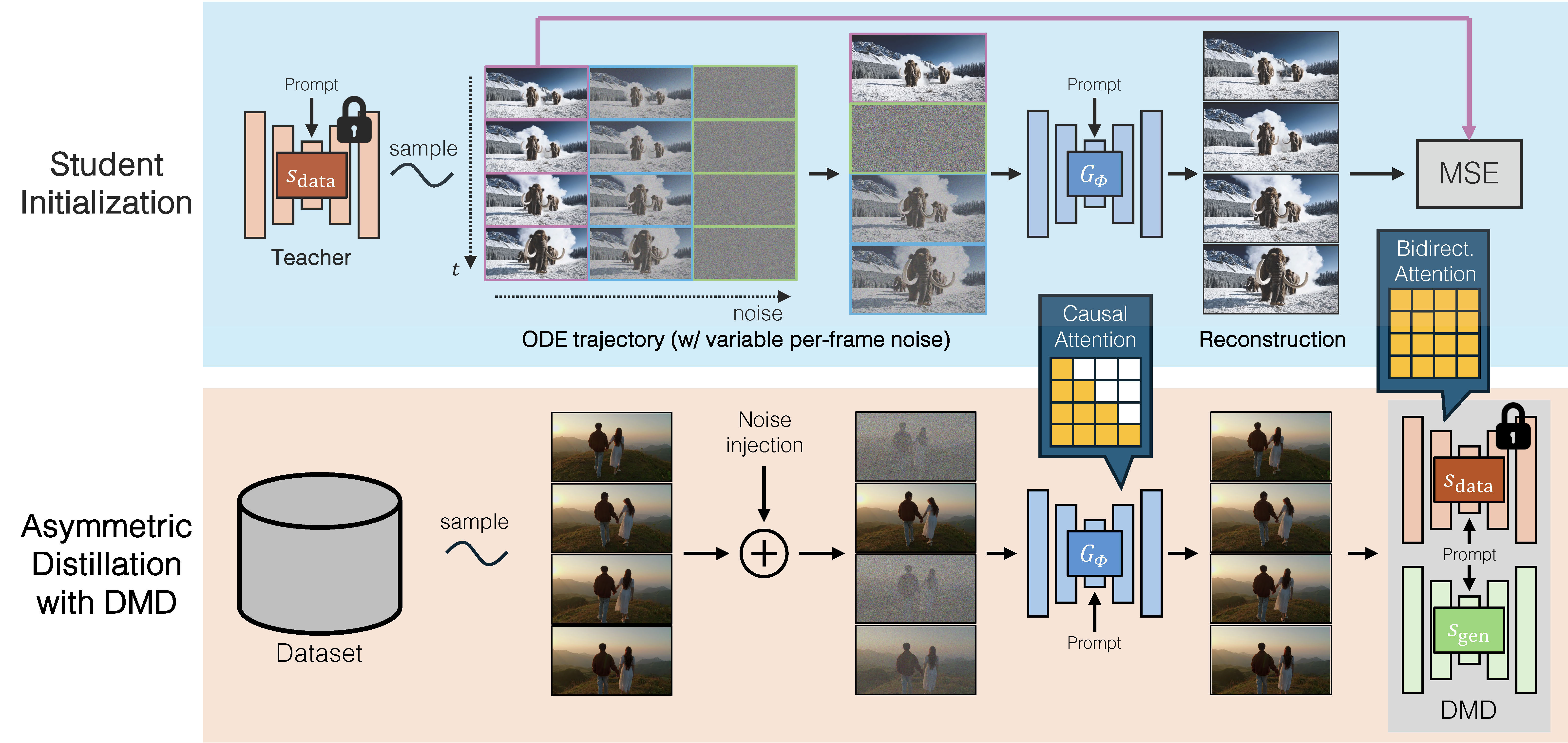
The solution from CausVid is elegant. Rather than naively fine-tuning a causal student on causal data, we use asymmetric distillation. The student has causal attention. The teacher retains bidirectional attention. The student learns to match the output distribution of the bidirectional teacher, not the behavior of a weaker causal teacher.
This asymmetric setup has a critical advantage. The bidirectional teacher does not suffer from error accumulation because it sees all frames simultaneously. When the causal student is trained to match this teacher’s distribution, it inherits this robustness, even though it will later generate frames sequentially. The teacher never makes the kinds of mistakes the student would make if it were trained on its own outputs.
The asymmetric distillation uses distribution matching loss (specifically DMD ) to align the student’s output distribution with the teacher’s. The key idea is that the gradient of the reverse KL divergence $D_{\text{KL}}(p_{\text{gen},t} \parallel p_{\text{data},t})$ at each noise level $t$ can be expressed as a difference of score functions:
where $G_\phi$ is the student generator, $\hat{x} = G_\phi(\epsilon)$ is the generated sample, $\hat{x}_t = \Psi(\hat{x}, t)$ is the noised version via the forward process from , $s_{\text{data}}$ is approximated by a pretrained bidirectional teacher, and $s_{\text{gen},\xi}$ is learned online using samples from the generator. This is equivalent to the following loss function:
where $\text{sg}[\cdot]$ denotes stop-gradient. The formulation allows the teacher and student to have entirely different attention patterns, which is critical for asymmetric (bidirectional→causal) distillation.
Once the causal student is trained, it can leverage KV caching for efficient inference. When generating frame $t+1$, all the key-value pairs from frames $1$ through $t$ are already computed and stored. Only the new frame’s queries need to attend to the cached keys and values. This reduces the time complexity from $O(N^2)$ (where $N$ is the sequence length) to $O(N)$ per new frame.
The result is dramatic. CausVid achieves 9.4 FPS on a single GPU with a first-frame latency of only 1.3 seconds, compared to 219 seconds for the bidirectional teacher to generate a 128-frame video. The causal model generates frames faster than video playback rate.
The Exposure Bias Problem
Converting a bidirectional model to causal is only half the battle. Autoregressive models face a fundamental challenge called exposure bias (also known as the train-test gap).
During training, the model predicts the next frame conditioned on ground-truth previous frames from the dataset. During inference, the model predicts the next frame conditioned on its own previous outputs. These are not the same distribution. The model has never seen its own mistakes during training, so it does not know how to recover from them.
Errors compound over time. A small artifact in frame 10 provides a corrupted input for generating frame 11. The corruption grows. By frame 50, the video may be unrecognizable. This is why early autoregressive video models produced quality that degraded rapidly with sequence length.

Three training strategies have been developed to address exposure bias, each with different tradeoffs.
Teacher Forcing
Teacher Forcing is the simplest approach where they train the model to denoise each frame conditioned on clean ground-truth previous frames. This is efficient and parallelizable (with appropriate masking), but the training distribution is far from the inference distribution. The model learns to generate the next frame assuming perfect context, which never happens during autoregressive inference.
Diffusion Forcing
Diffusion Forcing introduces a conceptually interesting idea; instead of treating noise level as a global property of the sequence, each token has an independent noise level. This treats noise as a continuous masking mechanism.
The key insight is that standard diffusion and next-token prediction are two extremes of the same spectrum. In full-sequence diffusion, all frames share the same noise level $k$. In next-token prediction, context frames are clean ($k = 0$) and the predicted frame is pure noise ($k = K$). Diffusion Forcing interpolates between these extremes.
The paper uses an RNN-based architecture where latent states $\mathbf{z}_t$ capture sequential dependencies. At each timestep $t$, the model receives the previous latent state $\mathbf{z}_{t-1}$ and a noisy observation $\mathbf{x}_t^{k_t}$ at noise level $k_t$. During training, each timestep’s noise level $k_t$ is sampled independently and uniformly from ${0, 1, \ldots, K}$. The training objective minimizes the noise prediction error:
where $k_{1{:}T} \sim \text{Uniform}([K]^T)$ and $\mathbf{z}_t$ is computed recurrently from previous states.
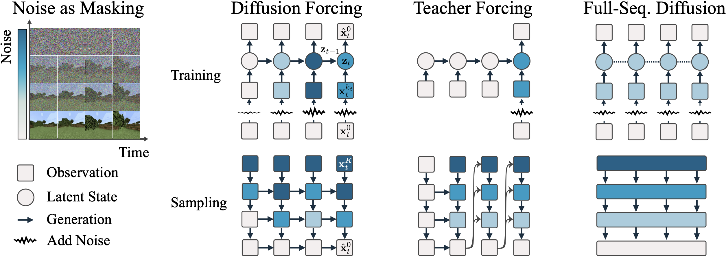
The insight is that noise acts as a continuous mask. Discrete masking (as in BERT or MAE) either reveals or hides a token. Noise provides soft, continuous masking where the token is partially revealed, with the degree of revelation controlled by the noise level. At $k = 0$, we have the clean token. As $k \to K$, the observation approaches pure Gaussian noise, conveying no information about the original.
Diffusion Forcing was shown to generate 2000+ frame videos (trained on only 36 frames) without sliding window inference and without quality collapse. However, it still does not fully match the inference distribution and the noisy context frames during training are noisy versions of ground truth, not noisy versions of model outputs. The model still never sees its own generation artifacts.
Self Forcing
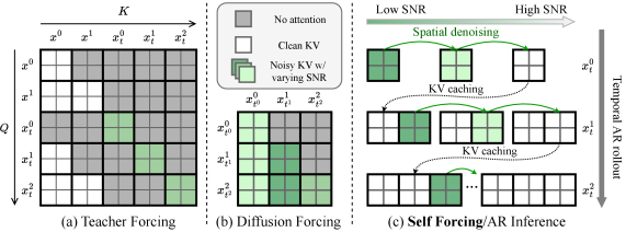
The key insight of Self Forcing is very simple. Instead of conditioning on ground-truth frames during training, condition on the model’s own generated frames. Perform the full autoregressive rollout during training, using KV caching, exactly as you would at inference time.
Formally, autoregressive video diffusion factorizes the joint distribution using the chain rule:
where each conditional $p(x_i \mid x_{<i})$ is modeled as a diffusion process. The forward process corrupts each frame independently:
where $t_i \in [0, 1000]$ can be sampled independently for each frame $i$.
This is computationally expensive if done naively. A 50-step diffusion model generating 100 frames would require 5000 forward passes, with gradients through all of them. The memory and compute requirements would be prohibitive.
Self Forcing addresses this through three design choices.
First, it uses a few-step diffusion model (4 steps instead of 50). The model distribution is implicitly defined as a composition of denoising steps:
where $f_{\theta, t_j}(x_{t_j}^i) = \Psi(G_\theta(x_{t_j}^i, t_j, x_{<i}), t_{j-1})$ and ${t_0 = 0, t_1, \ldots, t_T = 1000}$ is a subsequence of timesteps (typically $T = 4$ with a uniform schedule at $[1000, 750, 500, 250]$).
Second, it uses stochastic gradient truncation. At each training iteration, a random denoising step $s$ is sampled uniformly from ${1, 2, \ldots, T}$. Only the gradients from the $s$-th denoising step are propagated. Earlier steps are treated as fixed. This ensures all denoising steps receive supervision without requiring backpropagation through the entire chain.
Third, it detaches gradients across frames. The KV embeddings from previous frames are treated as constants when computing gradients for the current frame. This prevents gradient explosion from very long autoregressive chains.
Wan2.1-1.3B
SkyReels2-1.3B
CausVid-1.3B
Self Forcing-1.3B
With these modifications, Self Forcing training is surprisingly efficient. The per-iteration training time is comparable to Teacher Forcing and Diffusion Forcing. But the quality improvements are significant.
The training objective aligns the distribution of complete generated videos with the distribution of real videos. This is a holistic, video-level objective, not a frame-level one. Several distribution matching losses work well with Self Forcing.
DMD minimizes the reverse KL divergence $\mathbb{E}_t[D_{\text{KL}}(p_{\theta,t} \parallel p_{\text{data},t})]$ using the score difference gradient from .
SiD (Score Identity Distillation) minimizes the Fisher divergence:
where $f_\phi$ is the real score network and $f_\psi$ is the learned generator score. While $\alpha = 0.5$ theoretically corresponds to the Fisher divergence $\mathbb{E}_{t, p_{\theta,t}}[\parallel \nabla \log p_{\theta,t} - \nabla \log p_{\text{data},t} \parallel^2]$, the authors found that $\alpha = 1$ yields more stable training in practice.
GAN losses use R3GAN, which combines relativistic pairing with R1+R2 regularization:
where $x_t \sim p_{\text{data},t}$, $\hat{x}_t \sim p_{\theta,t}$, and the regularization encourages smooth discriminator outputs.
All three produce models with similar quality. The key is not which divergence you minimize, but that you minimize a divergence on the inference-time distribution, not the training-time distribution.
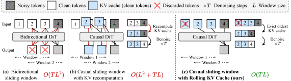
Self Forcing also introduces a rolling KV cache for long video generation. Bidirectional models require $O(TL^2)$ complexity since they cannot use KV caching. Prior causal models with KV recomputation have $O(L^2 + TL)$ complexity when the sliding window shifts. The rolling KV cache maintains a fixed-size buffer and discards the oldest entries as new frames are generated, achieving $O(TL)$ complexity for extrapolating videos beyond the training context length.
The result is a model that generates 17 FPS with 0.69 second latency (chunk-wise) or 8.9 FPS with 0.45 second latency (frame-wise) on a single H100 GPU. This is fast enough for real-time streaming applications.
MotionStream: Interactive Control and Infinite Length
Self Forcing closes the train-test gap for autoregressive video diffusion, but two challenges remain for truly interactive world models. First, how do you condition generation on user inputs that arrive continuously during inference, such as camera movements or object drags? Second, how do you maintain quality when generating beyond the training horizon into arbitrarily long sequences?
MotionStream addresses both. The goal is real-time, motion-controlled video generation that can run indefinitely with constant latency on a single GPU.
The architecture starts with a motion-conditioned teacher model. Each 2D track is represented as a $d$-dimensional sinusoidal embedding $\phi_n$ derived from a unique ID, placed at spatially downsampled locations in the conditioning signal $c_m \in \mathbb{R}^{T \times H/s \times W/s \times d}$. A lightweight track head (just 4× temporal compression plus a 1×1×1 convolution) processes these embeddings before concatenation with video latents. This is far more efficient than ControlNet-style architectures that duplicate network blocks.
The teacher is trained with rectified flow matching on the velocity field $v_\theta(z_t, t, c_t, c_m)$, where $c_t$ is the text prompt and $c_m$ is the motion condition. A key design choice is joint text-motion guidance:
where $v_{\text{base}} = \alpha \cdot v(\varnothing, c_m) + (1-\alpha) \cdot v(c_t, \varnothing)$ and $\alpha = w_t/(w_t + w_m)$. Text guidance provides natural dynamics (weather changes, secondary motions) while motion guidance enforces precise trajectory adherence. Pure motion guidance produces overly rigid 2D translations. Pure text guidance loses trajectory fidelity. Their combination (with $w_t = 3.0$, $w_m = 1.5$) balances both.

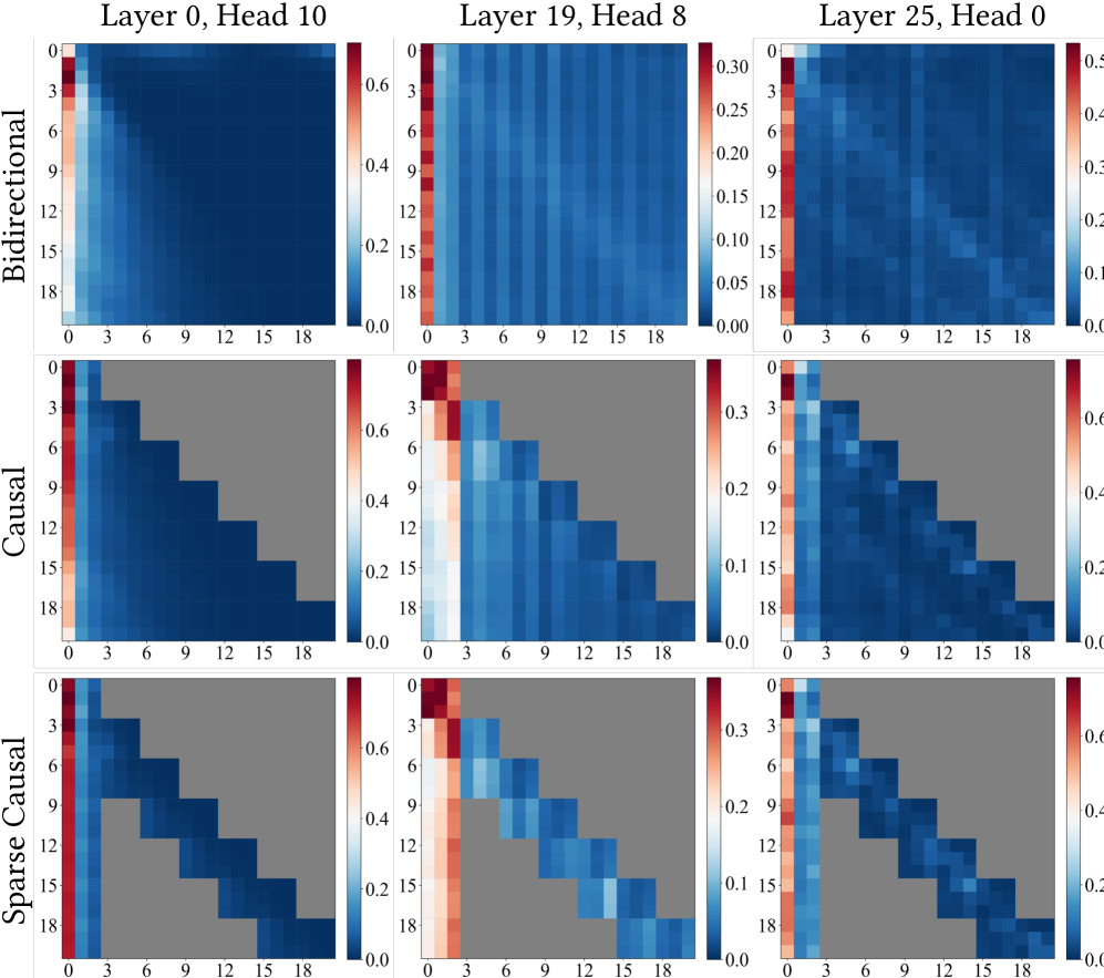
The causal student is distilled using Self Forcing with DMD. But naively applying Self Forcing to motion-controlled generation reveals a problem where quality degrades rapidly when extrapolating beyond the teacher’s training horizon (81 frames). Analyzing attention maps provides the explanation.
Many attention heads persistently focus on tokens from the initial frame throughout generation, even as the context window shifts. This mirrors the “attention sink” phenomenon observed in StreamingLLM for language models, where the first few tokens absorb disproportionate attention mass regardless of their semantic content. In video, the initial frame serves as an anchor that stabilizes generation.
MotionStream exploits this by maintaining $S$ sink chunks from the initial frame alongside a local window of $W$ recent chunks. The context for denoising chunk $i$ becomes:
where $z_t^i$ is the current noisy chunk and $z_0^j$ are previously generated clean chunks. The sink tokens use frozen RoPE positions (computed once at initialization), while window tokens receive dynamic positions based on their current cache location. This creates a temporal discontinuity between sink and window that the model learns to handle during training.
Crucially, MotionStream trains with the same attention sink and rolling KV cache configuration used at inference. This extrapolation-aware training eliminates the train-test gap for long sequences. The teacher evaluates continuous video frames (no temporal discontinuity), providing robust score targets. The student learns to handle the sink-window discontinuity because it appears identically during training.
The DMD gradient for the causal student incorporates joint guidance directly:
where $s_{\text{real}}$ uses the frozen teacher with joint guidance (requiring 3 NFE per step), while $s_{\text{fake}}$ is a trainable critic without CFG. This “bakes” the expensive multi-term guidance into the distillation objective, allowing the student to replicate joint-guided quality with a single function evaluation.
Experiments reveal that minimal configurations work best. A single sink chunk ($S = 1$) with a single-chunk local window ($W = 1$) outperforms larger windows during long-video extrapolation. Additional sink chunks provide marginal gains while increasing latency. Larger windows actually degrade quality because attending to long-past history allows errors to accumulate in context tokens. The minimal configuration forces the model to compress all relevant history into the immediate predecessor and initial anchor.
For maximum speed, MotionStream introduces a Tiny VAE decoder trained with adversarial loss and LPIPS regression against the original VAE’s latent space. This reduces decoding time by over 10×, removing the VAE bottleneck that otherwise consumes 35-47% of wall time. The final system achieves 17 FPS at 480p with full VAE (0.69s latency) or 29.5 FPS with Tiny VAE (0.39s latency) on a single H100. For 720p, the numbers are 10.4 FPS and 23.9 FPS respectively. On motion transfer benchmarks, MotionStream matches or exceeds prior offline methods (Go-With-The-Flow, Diffusion-As-Shader) while being 20-40× faster.
The limitation is that attention sinks anchor generation to the initial scene. For applications requiring complete scene changes (game world exploration where environments continuously change), the model tends to preserve initial features rather than adapting to new contexts. This is a fundamental constraint of the track-based conditioning, which cannot meaningfully encode full scene transitions.
Accelerating Diffusion with Distribution Matching
The speed improvements in CausVid and Self Forcing rely heavily on reducing the number of denoising steps. Standard diffusion requires 50-100 steps; few-step diffusion achieves comparable quality in 4 steps. This compression is enabled by distribution matching distillation.
The key idea, introduced in DMD , is to minimize the KL divergence between the generated and target distributions at the output level, rather than matching individual denoising steps.
Recall that the score function relates to the noise prediction via $s_\theta(x_t, t) = -\epsilon_\theta(x_t, t)/\sigma_t$ (from ). The gradient of the reverse KL divergence can be written as:
The second term $\nabla_\phi \log p_{\text{gen},t}(x_t)$ is handled through the reparameterization trick. For a generator $G_\phi(\epsilon)$ with $\epsilon \sim \mathcal{N}(0, I)$, after applying the forward process and taking expectations:
where $\hat{x} = G_\phi(\epsilon)$, $\hat{x}_t = \Psi(\hat{x}, t)$, and $\omega(t)$ is a weighting function.
The score $s_{\text{data}}$ pulls the generator output toward real data. The score $s_{\text{gen}}$ pushes away from the generator’s current distribution. Together they form a gradient that moves the generator’s distribution toward the data distribution.
DMD2 extends this to multi-step generation by replacing the pure noise input $\epsilon$ with a partially denoised intermediate $x_t$. It also introduces the two-timescale update rule, where the generator $G_\phi$ is updated more frequently than the online score network $s_{\text{gen},\xi}$. Specifically, the ratio is typically 5:1, which stabilizes training by preventing the fake score network from adapting too quickly to generator changes.
What makes DMD particularly suitable for causal video generation is that the teacher and student can have different architectures. The teacher can be bidirectional (higher quality, slower). The student can be causal (lower quality without distillation, but fast with KV caching). The distribution matching objective only requires samples from both; it does not require the architectures to match.
This flexibility is crucial. A causal teacher would suffer from the same error accumulation as the student. By using a bidirectional teacher, we transfer the teacher’s robustness to the student without requiring the student to be bidirectional.
Memory for Minutes: Mixture of Contexts
Attention is quadratic in sequence length. A minute-long 480p video at 12 FPS, after VAE compression (16× spatial, 4× temporal downsampling), becomes a sequence of approximately 180,000 tokens. Standard self-attention over this sequence becomes computationally intractable. For even longer videos, the numbers become astronomical.
Sparse attention is the natural solution, but which tokens should attend to which? Fixed sparsity patterns (local windows, strided attention) cannot adapt to the content. A reference to an object that appeared 30 seconds ago requires attending to those specific frames, not a fixed window. Prior methods either compress history into lossy summaries (keyframes, latent states) or impose static sparse patterns that cannot adapt to which past events matter at each step.
Mixture of Contexts (MoC) reframes long-context video generation as an internal information retrieval problem. Rather than attending to all context or using fixed sparsity, each query token dynamically selects only the most relevant chunks of context through a learned sparse attention routing mechanism.
The key insight is that video data exhibits high temporal redundancy, and spatially/temporally adjacent tokens often represent redundant or correlated visual elements. MoC partitions the multi-modal token stream into content-aligned chunks along natural boundaries (frames, shots, and modality stripes) rather than fixed-length windows. This ensures each chunk is semantically homogeneous, making the routing signal more discriminative.
For every query token $q_i$, MoC computes a relevance score against each chunk using a parameter-free router: it takes the dot product between $q_i$ and a mean-pooled descriptor $\phi(K_\omega) = \text{mean}(K_\omega)$ of each chunk’s keys. The top-$k$ most relevant chunks are selected:
where $\Omega(q_i)$ is the set of indices for the top-$k$ selected chunks. The mean-pooling descriptor is remarkably effective because, as shown in prior work on denoising diffusion autoencoders, diffusion transformers learn semantically meaningful representations where the mean of a token chunk effectively captures its dominant semantic content.
Crucially, the router is parameter-free yet trainable. While the top-$k$ selection itself is non-differentiable, the model learns indirectly through the attention mechanism on selected chunks. If a selected chunk proves irrelevant, gradients from the loss flow back through its keys/values, attenuating unhelpful representations and encouraging more discriminative query/key projections over training.
MoC introduces several design elements that ensure robust routing:
- Mandatory anchors: Every visual query always attends to (1) all text/caption tokens (providing semantic grounding) and (2) tokens within the same shot (ensuring local coherence). This reserves routing capacity for genuinely long-range recall.
- Causal routing: To prevent pathological feedback loops where chunk $i$ routes to chunk $j$ while $j$ routes back to $i$, MoC imposes a causal mask restricting each chunk to attend only to earlier positions, transforming the routing graph into a directed acyclic graph.
- Per-head distributed routing: Rather than selecting a global set of chunks for the entire network, routing operates independently for each attention head in every layer. Different heads specialize in distinct feature subspaces, and the union of selected chunks across all heads covers a large portion of the context.
- Context drop-in/drop-out: During training, randomly removing selected chunks (drop-out) and injecting extraneous chunks (drop-in) promotes robustness to routing errors and prevents “dead route” problems analogous to dead experts in Mixture-of-Experts systems.
MoC achieves dramatic efficiency gains. For 8-shot, minute-long scenes with approximately 180,000 tokens, MoC prunes about 85% of token pairs and reduces attention FLOPs by over 7×, yielding a measured 2.2× end-to-end generation speedup. Importantly, this sparsity does not compromise quality—the model often improves on metrics like Dynamic Degree (motion diversity) while maintaining consistency, because compute is reallocated from redundant frames to salient visual events.
This connects to a deeper insight about video structure. Videos are not uniformly dense in information. Long static shots contain redundant frames. Key events (scene transitions, object appearances, action changes) carry disproportionate information. A good video model should allocate attention according to information content, not uniform temporal distance. MoC learns this allocation end-to-end, without explicit heuristics like Field-of-View overlapping or 3D geometric priors.
Beyond Pixels: Latent Space World Models
A recurring theme in the papers discussed so far is that generation happens in latent space. A 3D VAE compresses video frames into shorter sequences of latent tokens. The diffusion model operates on these latents. A decoder converts latents back to pixels.
This design has several advantages. Latents are lower-dimensional than pixels, so diffusion is cheaper. Latents are more semantically meaningful, so learning is easier. Compression removes perceptually irrelevant details, focusing the model on structure.
But there is a deeper question. For world modeling, do we even need to predict pixels? If the goal is planning, control, or understanding, we only need a representation that supports downstream tasks. Predicting full RGB frames may be wasteful.
V-JEPA 2 takes this direction to the extreme. It predicts in the latent space of a pretrained DINOv2 encoder, never touching pixels at all. The model learns an action-conditioned world model from internet video, predicting how latent representations evolve given actions.
This latent-space prediction has advantages for control. The latent space is invariant to irrelevant visual details (lighting changes, textures). Planning in this space focuses on task-relevant structure.
DINO-world similarly operates in DINOv2 latent space, showing strong intuitive physics understanding. Objects that should move together do move together. Occlusion is handled correctly. Physical plausibility emerges from prediction in a semantically rich latent space.
The tradeoff is that these models cannot generate photorealistic video. They predict abstract representations, not renderable frames. But for world modeling applications (robotics, planning, simulation), this may not matter.
4D World Models: Geometry and Dynamics Together
Video is a 2D projection of a 3D world evolving in time. Standard video models treat frames as images, ignoring the underlying 3D structure. This leads to problems.
When the camera moves, a 2D video model must learn to reproject the scene from scratch. It does not know that rotating the camera by 10 degrees should produce a consistent view of the same 3D objects. Hallucinating consistent 3D structure from pure 2D supervision is hard.
4D world models address this by jointly predicting 3D structure and dynamics. Instead of outputting RGB frames, they output representations that decompose into geometry (depth, normals) and appearance (color, texture).
TesserAct predicts RGB, depth, and surface normals (RGB-DN) jointly. The model is trained on videos with ground-truth depth (from simulation or RGBD sensors) and learns to predict all three modalities together. At inference, it can render novel views by reprojecting the predicted depth.
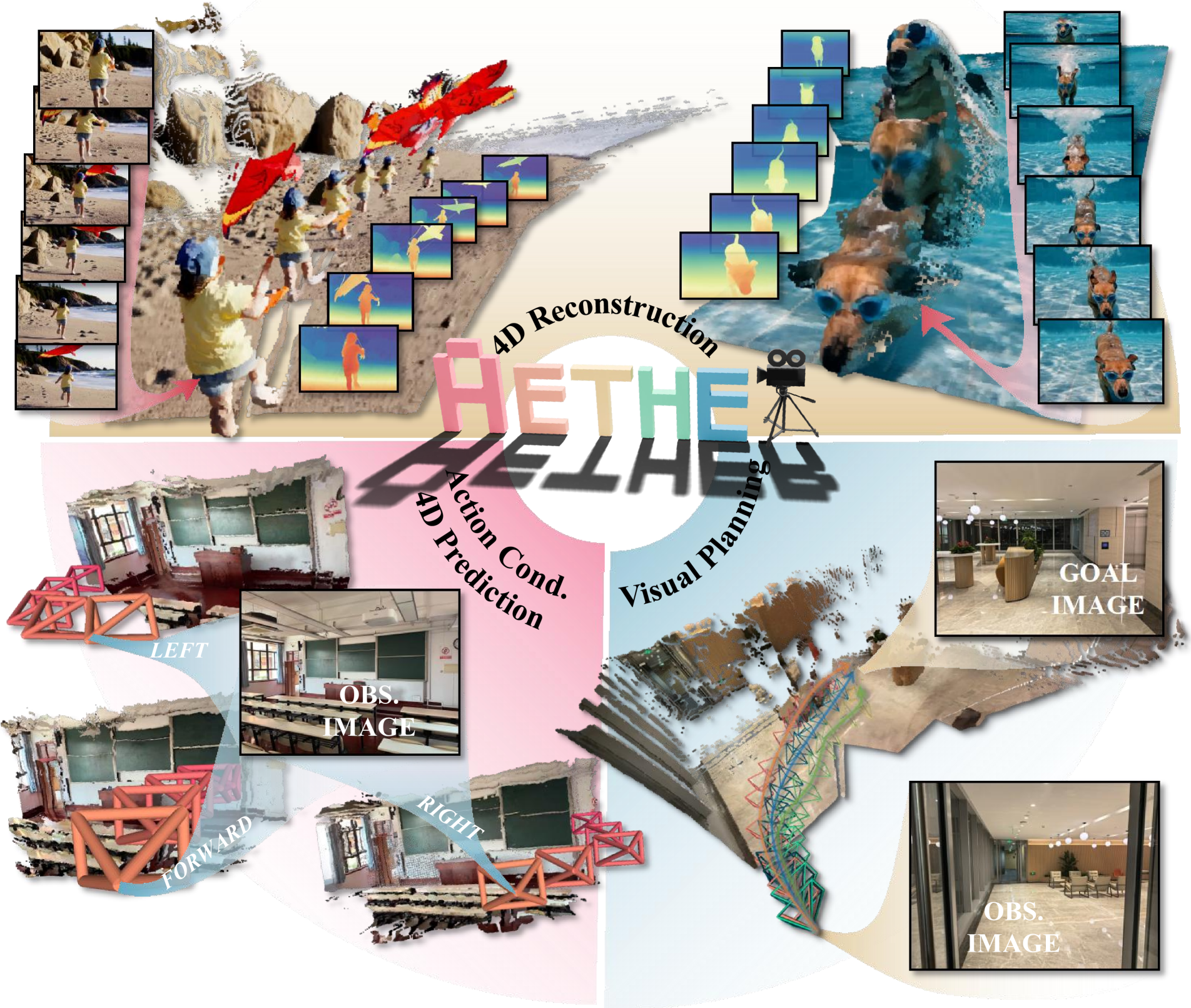
Aether provides a unified framework for 4D dynamic reconstruction, action-conditioned video prediction, and goal-conditioned visual planning. The key insight is that these tasks share the same underlying representation. A model that understands 4D dynamics can perform all three.
The geometry-aware representation has several benefits. View synthesis is possible by reprojecting predicted depth to novel cameras. Physical reasoning is easier when the model knows about 3D structure. Generalization improves because the model learns about the 3D world, not just 2D patterns.
The price is that training requires 3D supervision (depth, normals, camera poses), which is more expensive to collect than RGB video. But the resulting models are more capable world simulators.
General World Models: Toward Unified Architectures
The papers discussed so far focus on specific aspects of the world modeling problem. A natural question is whether we can build a single model that handles all aspects.
PAN (Perception-Action Navigation) combines an autoregressive LLM backbone with a video diffusion decoder. The LLM predicts compact latent actions and physics states. The diffusion decoder renders these predictions as video frames. This separation allows the model to reason about dynamics at a high level while delegating appearance generation to a specialized component.
The architecture is called Generative Latent Prediction (GLP). The LLM operates on a sequence of latent tokens, one per frame. Each latent encodes the “state” of the world at that timestep. The diffusion decoder conditions on these latents to produce the actual RGB frames.
This design addresses the mismatch between discrete, symbolic reasoning (where LLMs excel) and continuous, perceptual generation (where diffusion excels). The LLM handles planning and physics. The diffusion model handles appearance.
What Makes a World Model?
Let me step back and ask a deeper question. What distinguishes a world model from a video generator?
A video generator produces plausible video given a prompt. It may hallucinate objects that do not exist, violate physics, or generate inconsistent geometry. These are acceptable if the goal is entertainment or illustration.
A world model must do more. It must obey the constraints of the world it models. Objects have persistent identities. Actions have causal consequences. Physics is (mostly) conserved.
The papers discussed here represent different approaches to learning these constraints.
Causal attention enforces temporal causality. The future cannot influence the past.
Self Forcing enforces consistency with the model’s own outputs. The model must handle its own mistakes.
Attention sinks enforce stable long-term generation. Anchoring to initial frames prevents drift during infinite-length rollouts.
Distribution matching enforces consistency with real video. Generated videos must be indistinguishable from real ones.
Sparse attention (MoC) enforces selective memory. The model must learn what past information is relevant.
4D prediction enforces geometric consistency. The 3D world must be coherent across views.
None of these alone creates a full world model. Together, they provide a foundation.
Looking Forward
The field is moving fast. Several directions seem particularly promising.
Longer context windows are needed to capture the temporal structure of real activities. Current models handle seconds to minutes. Real tasks (cooking, assembly, navigation) unfold over hours.
Better memory mechanisms will be required. Mixture of Contexts is a step, but we likely need more structured representations. State-space models, persistent external memory, and retrieval-augmented generation are all possibilities.
Unified training objectives that combine generation, prediction, and planning would avoid the current fragmentation. A model trained only on generation may not understand causality. A model trained only on prediction may not generate high-quality samples.
Better evaluation is needed. Current benchmarks (VBench, FVD) focus on visual quality and text alignment. They do not measure physical plausibility, long-term consistency, or controllability.
Scaling laws for video world models are not well understood. Do these models scale like LLMs? Do they benefit from video-specific architectural choices? How much compute is needed for useful world simulators?
Conclusion
The path from bidirectional video diffusion to autoregressive world models requires solving several interconnected problems. Causality must be imposed through attention masking. Error accumulation must be addressed through self-forcing or distribution matching. Inference must be accelerated through distillation and KV caching. Memory must be efficient through sparse attention. And for true world modeling, geometry and physics must be incorporated into the representation.
Each of the papers discussed here solves one piece of the puzzle. CausVid shows how to convert bidirectional to causal. Self Forcing bridges the train-test gap. MotionStream adds interactive control and attention sinks for infinite-length streaming. DMD2 enables few-step generation. Diffusion Forcing provides flexible noise scheduling. Mixture of Contexts enables long-range memory. TesserAct and Aether incorporate 4D structure.
The goal of photorealistic, real-time, physically plausible world simulation remains distant. But the trajectory is clear. Video generation is becoming video prediction. Video prediction is becoming world modeling. And world modeling is becoming a foundation for embodied AI.